Introduction to Violin Plots with Vega-Lite

Author

Affiliation

Mike Travers

Scicloj

Published

February 3, 2026

The World’s Smallest Violin (plot generating code)

This post explains how to visualize data with violin plots, using Vega-Lite and Clojure.

What is a violin plot?

A Violin plot is a way to visualize how data is distributed - essentially showing you where your data points fall and how spread out they are.is

Imagine you’re analyzing a dataset of movies and how much money they made. A violin plot would show you not just the median value, but the full “shape” of your data: Are values clustered around certain points, ore evenly spread out? How much concentration is there? How many such points?

A violin plot is best understood as an extension of the more common box plot. Violin plots add a visulization of the probability density, and can reveal more features of the data, such as multiple modes. This tutorial shows you how to make box plots and violin plots in Vega-Lite.

Violin plots are common in the scientific literature. For an example of using violin plots in a scientific domain, see the BRUCE website, which uses interactive violin plots to visualize data from a brain cancer research project.

References

Violin Plots: A Box Plot-Density Trace Synergism Jerry L. Hintze, Ray D. Nelson
Violin Plot - Wikipedia

Resources

A miminal Clojure project for generating Vega plots
Vaguely Vaguely, a block-based environment for experimenting with Vega
Vega-Lite The Vega documentation
Hanami), a templating library for generating Vega plots in Clojure

Data

We’ll use this classic dataset about penguin morphology. Each row in this dataset describes an individual penguin, with properties like species, sex, body mass, wing size.

(def penguin-data-url
  "https://raw.githubusercontent.com/ttimbers/palmerpenguins/refs/heads/file-variants/inst/extdata/penguins.tsv")

(def penguin-data
  (tc/dataset penguin-data-url {:key-fn keyword}))

(kind/table
 (tc/random penguin-data 10))

species island	bill_length_mm	bill_depth_mm	flipper_length_mm	body_mass_g	sex	year
Adelie Biscoe	42.0	19.5	200	4050	male	2008
Gentoo Biscoe	46.9	14.6	222	4875	female	2009
Adelie Torgersen	38.8	17.6	191	3275	female	2009
Chinstrap Dream	45.9	17.1	190	3575	female	2007
Gentoo Biscoe	50.5	15.2	216	5000	female	2009
Adelie Dream	37.3	16.8	192	3000	female	2009
Adelie Dream	40.7	17.0	190	3725	male	2009
Gentoo Biscoe	43.5	14.2	220	4700	female	2008
Gentoo Biscoe	52.2	17.1	228	5400	male	2009
Adelie Torgersen	35.7	17.0	189	3350	female	2009

Just show me the datapoints

Let’s start off with a simple dot-plot. We’ll group the data by species, and turn each value for body_mass into a point. Vega just requires specifying some basic mappings (aka encodings) between data fields and visual properties. So a minimal dot plot can look like this:

^:kind/vega-lite
{:mark {:type "point"}
 :data {:values (tc/rows penguin-data :as-maps)}
 :encoding
 {:x {:field "body_mass_g"
      :type :quantitative}
  :y {:field "species island"
      :type :nominal}}
 }

Vega’s defaults are not always what we want, so the next version has the same as structure as before, with a bit of tweaking to look more like what we want. We’ll adjust the size of the graph, adjust the scale, use color. We add some randomness (jitter) so we can better see individual points, and just for the hell of it, map another attribute, sex, to :shape.

^:kind/vega-lite
{:mark {:type "point" :tooltip {:content :data}}
 :data {:values (tc/rows penguin-data :as-maps)}
 :transform [{:calculate "random()" :as "jitter"}]
 :encoding
 {:x {:field "body_mass_g"
      :type :quantitative
      :scale {:zero false}}
  :row {:field "species island"
        :type :nominal
        :header {:labelAngle 0 :labelAlign "left"}
        :spacing 0}
  :color {:field "species island"
          :type :nominal
          :legend false}
  :shape {:field "sex"
          :type :nominal}
  :y {:field "jitter"
      :type :quantitative
      :axis false}}
 :height 50                             ;Note: this specifies the height of a single row 
 :width 800
 }

One nonobvious change: we use :row in place of :y for the group (species) dimension. This is not estrictly necessary at this point, but will make it easier when we get to actual violin plots. Just to be more confusing, we reuse the :y encoding for the random jitter.

Boxplot

A boxplot is another way of displaying the distribution of a single numeric varianle. A box plot summarizes a distribution of quantitative values using a set of summary statistics. The median tick in the box represents the median. The left and right parts of the box represent the first and third quartile respectively. The whisker shows the full domain of the data.

^:kind/vega-lite
{:mark {:type :boxplot
        :extent :min-max}
 :data {:values (tc/rows penguin-data :as-maps)}
 :encoding
 {:x {:field "body_mass_g"
      :type :quantitative
      :scale {:zero false}}
  :y {:field "species island"
      :type :nominal}
  :color {:field "species island"
          :type :nominal
          :legend false}}
 :height {:step 50}
 :width 800
 }

Violin Plot

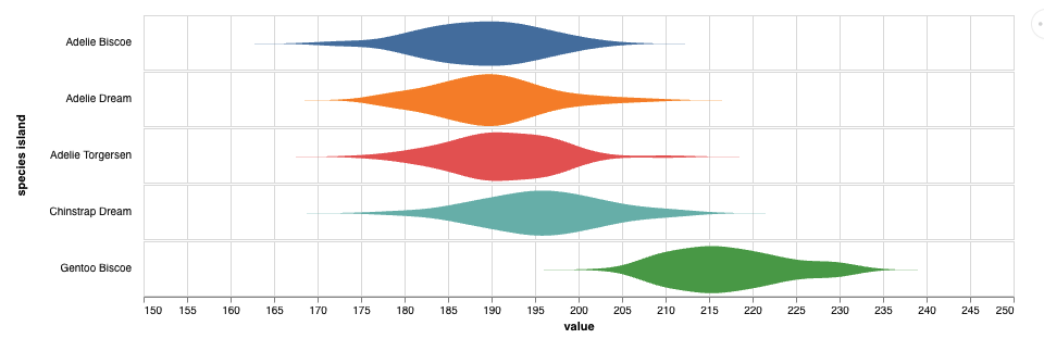
Violin plots extend the idea of a box plot. The basic geometry is the same, but instead of showing just a few coarse statistics like median, a violin plot shows the probability density as a continuous variable.

Vega-lite provides a :density transform that does the work of computing this. This transform has a number of options; :bandwidth controls the degree of smoothing of the density curve, and you can select a value depending on your data and needs.

(kind/vega-lite
 {:mark {:type :area}
  :data {:values (tc/rows penguin-data :as-maps)}
  :transform [{:density "body_mass_g"
               :groupby ["species island"]
               :bandwidth 80}]
  :encoding
  {:color {:field "species island"
           :type :nominal
           :legend false}
   :x {:field "value"
       :title "body_mass_g"
       :type :quantitative
       :scale {:zero false}}
   :y {:field "density"
       :type :quantitative
       :stack :center                   ; this reflects the area plot to produce the violin shape. 
       :axis false                      ; hide some labels
       } 
   :row {:field "species island"
         :type :nominal
         :spacing 0
         :header {:labelAngle 0 :labelAlign :left}
         }
   }
  :height 50                            ;this is the height of each row (facet)
  :width 800
  })

That’s the basics of a violin plot! In Part 2, we’ll see about abstracting some of this into functions, with some variations. and we’ll look at combining violin plots with dot and box plots for a richer of our data.

source: src/data_visualization/violin.clj