Image Processing with dtype-next Tensors

Author

Affiliations

Published

December 10, 2025

Introduction: Why dtype-next for Image Processing?

Images are perfect for learning dtype-next because they’re typed numerical arrays with clear visual feedback. Unlike generic sequences where numbers are boxed, dtype-next gives us:

Efficient storage: A 1000×1000 RGB image is 3MB of uint8 values, not 12MB+ of boxed objects
Zero-copy views: Slice channels, regions, or transforms without copying data
Functional operations: Element-wise transformations that compose naturally
Type discipline: Explicit control over precision and overflow

What Are Tensors?

A tensor is a multi-dimensional array of numbers with a defined shape and type. While the term comes from mathematics and physics, in programming it simply means: structured numerical data with multiple axes.

A scalar is a 0D tensor (single number)
A vector is a 1D tensor [5] → 5 elements
A matrix is a 2D tensor [3 4] → 3 rows × 4 columns
An RGB image is a 3D tensor [height width 3] → spatial dimensions + color channels
A video is a 4D tensor [time height width 3] → adding a time axis

Tensors provide efficient storage (typed, contiguous memory) and convenient multi-dimensional indexing. Operations on tensors (slicing, element-wise math, reductions) form the foundation of numerical computing, from image processing to machine learning.

About This Tutorial

dtype-next is a comprehensive library for working with typed arrays, including buffers, functional operations, tensors, and dataset integration. This tutorial focuses on the tensor API—multi-dimensional views over typed buffers—because images provide clear visual feedback and natural multi-dimensional structure.

The patterns you’ll learn (zero-copy views, type discipline, functional composition) transfer directly to other dtype-next use cases: time series analysis, scientific computing, ML data preparation, and any domain requiring efficient numerical arrays.

What We’ll Build

Working with Tensors — reshaping, dataset conversion, core operations
Tensor Operations Primer — slicing, element-wise ops, type handling
Image Statistics — channel means, ranges, distributions, histograms
Spatial Analysis — gradients, edge detection, sharpness metrics
Enhancement Pipeline — white balance, contrast adjustment
Accessibility — color blindness simulation
Convolution & Filtering — blur, sharpen, Sobel edge detection
Downsampling & Multi-Scale Processing — pyramids, multi-resolution analysis

Each section demonstrates core dtype-next concepts with immediate practical value.

Setup: Loading Images as Tensors

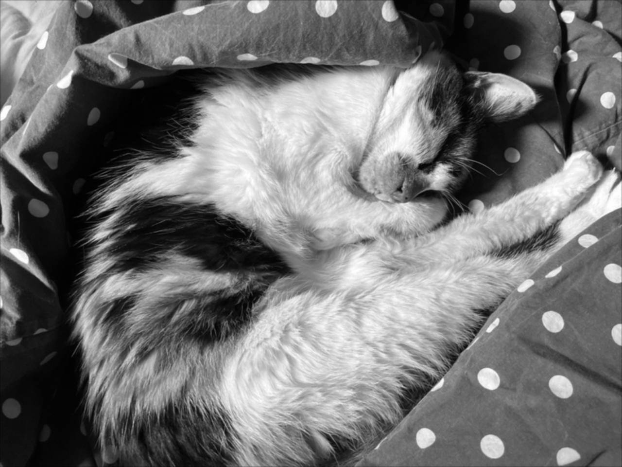
Let’s load our sample image and understand the tensor structure.

The bufimg Namespace

(require '[tech.v3.libs.buffered-image :as bufimg])

The tech.v3.libs.buffered-image namespace (aliased as bufimg) provides interop between Java’s BufferedImage and dtype-next tensors:

bufimg/load — load image file → BufferedImage
bufimg/as-ubyte-tensor — BufferedImage → uint8 tensor [H W C]
bufimg/tensor->image — tensor → BufferedImage (for display)

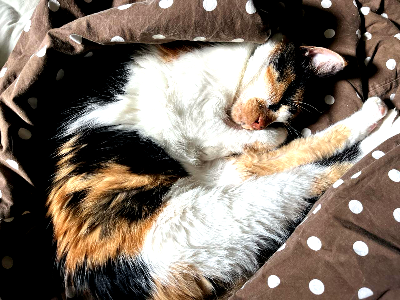
(def original-img
  (bufimg/load "src/dtype_next/nap.jpg"))

original-img

(def original-tensor
  (bufimg/as-ubyte-tensor original-img))

⚠️ Important: Understanding Channel Order

BufferedImage can use different pixel formats (RGB, BGR, ARGB, etc.). The specific format depends on the image type and how it was loaded. Our image uses BGR order:

(bufimg/image-type original-img)

:byte-bgr

:byte-bgr means this image stores colors in BGR (Blue-Green-Red) order, not RGB. The bufimg/as-ubyte-tensor function preserves whatever order BufferedImage uses.

For this tutorial’s BGR images, the channels are:

Channel 0 = Blue
Channel 1 = Green
Channel 2 = Red

Always check bufimg/image-type to confirm your image’s channel order before processing. We’ll be explicit about BGR ordering throughout this tutorial.

Why the round-trip works: bufimg/tensor->image defaults to creating BGR BufferedImages. So our workflow maintains BGR throughout: load BGR → process as BGR tensor → create BGR image. If you had an RGB tensor, you’d need to either swap channels or use (bufimg/tensor->image rgb-tensor {:img-type :int-rgb}).

original-tensor

#tech.v3.tensor<uint8>[960 1280 3]
[[[163 173 173]
  [169 179 179]
  [176 186 186]
  ...
  [ 58  74  87]
  [ 53  69  82]
  [ 51  67  80]]
 [[165 175 175]
  [170 180 180]
  [176 186 186]
  ...
  [ 59  75  88]
  [ 59  75  88]
  [ 58  74  87]]
 [[165 175 175]
  [168 178 178]
  [172 182 182]
  ...
  [ 54  70  83]
  [ 53  69  82]
  [ 50  66  79]]
 ...
 [[ 79  87  94]
  [ 73  81  88]
  [ 67  75  82]
  ...
  [ 78  89 109]
  [ 78  89 109]
  [ 78  89 109]]
 [[ 83  91  98]
  [ 78  86  93]
  [ 75  83  90]
  ...
  [ 78  89 109]
  [ 78  89 109]
  [ 78  89 109]]
 [[ 89  97 104]
  [ 84  92  99]
  [ 82  90  97]
  ...
  [ 78  89 109]
  [ 78  89 109]
  [ 78  89 109]]]

Understanding Tensor Shape

(require '[tech.v3.datatype :as dtype])

The tech.v3.datatype namespace provides core functions for inspecting and manipulating typed data.

Shape tells us dimensions:

(dtype/shape original-tensor)

[960 1280 3]

This is [height width channels] — our image has 3 color channels.

(def height
  (first (dtype/shape original-tensor)))

(def width
  (second (dtype/shape original-tensor)))

Element type:

(dtype/elemwise-datatype original-tensor)

:uint8

:uint8 means each pixel component is an unsigned byte (0-255).

Total elements:

(dtype/ecount original-tensor)

That’s height × width × 3.

Working with Tensors

Before diving into image analysis, let’s understand what tensors are in dtype-next.

Tensors are multi-dimensional views over typed buffers. The underlying buffer is a contiguous block of typed data (like our uint8 pixels), and the tensor provides convenient multi-dimensional indexing with shape information. This architecture enables zero-copy operations—when we slice or reshape, we create new views without copying data.

Let’s explore essential tensor operations for transforming and converting data.

Reshaping

Sometimes it’s convenient to flatten spatial dimensions into a single axis. For example, reshaping [H W 3] → [H×W 3] gives us one row per pixel:

(-> original-tensor
    (tensor/reshape [(* height width) 3])
    dtype/shape)

[1228800 3]

Key insight: tensor/reshape is a zero-copy view operation—it reinterprets the buffer without copying data.

Tensors as Datasets

(require '[tech.v3.dataset.tensor :as ds-tensor])

(require '[tablecloth.api :as tc])

The tech.v3.dataset.tensor namespace provides conversions between tensors and datasets. The tablecloth.api namespace of Tablecloth also auto-converts 2D tensors.

Two-dimensional tensors convert naturally to tablecloth datasets, enabling tabular operations and plotting.

Converting tensors ↔︎ datasets:

ds-tensor/tensor->dataset — explicit conversion
tc/dataset — tablecloth auto-converts 2D tensors
ds-tensor/dataset->tensor — convert back to tensor

(-> original-tensor
    (tensor/reshape [(* height width) 3])
    ds-tensor/tensor->dataset
    (tc/rename-columns [:blue :green :red]))

:_unnamed [1228800 3]:

:blue	:green	:red
163	173	173
169	179	179
176	186	186
182	192	192
186	196	196
189	199	199
193	203	203
195	205	205
198	208	208
198	208	208
…	…	…
80	91	111
79	90	110
79	90	110
79	90	110
79	90	110
79	90	110
78	89	109
78	89	109
78	89	109
78	89	109
78	89	109

Or more concisely (tablecloth auto-converts):

(-> original-tensor
    (tensor/reshape [(* height width) 3])
    tc/dataset
    (tc/rename-columns [:blue :green :red]))

:_unnamed [1228800 3]:

:blue	:green	:red
163	173	173
169	179	179
176	186	186
182	192	192
186	196	196
189	199	199
193	203	203
195	205	205
198	208	208
198	208	208
…	…	…
80	91	111
79	90	110
79	90	110
79	90	110
79	90	110
79	90	110
78	89	109
78	89	109
78	89	109
78	89	109
78	89	109

We can convert back, restoring the original image structure:

(-> original-tensor
    (tensor/reshape [(* height width) 3])
    tc/dataset
    ds-tensor/dataset->tensor
    (tensor/reshape [height width 3])
    bufimg/tensor->image)

Creates BGR BufferedImage by default

This round-trip demonstrates the seamless interop between tensors and datasets, useful for combining spatial operations (tensors) with statistical analysis (datasets).

Tensor Operations Primer

Before working with real images, let’s explore the core operations we’ll use throughout this tutorial. We’ll use tiny toy tensors to demonstrate each concept.

Creating Tensors: tensor/compute-tensor

(require '[tech.v3.tensor :as tensor])

The tech.v3.tensor namespace provides multi-dimensional array operations.

tensor/compute-tensor creates a tensor by calling a function for each position. The function receives indices and returns the value for that position.

Buffers, Readers, and Writers

Before working with tensors, let’s understand dtype-next’s foundational abstractions. These concepts will help us understand what happens when we slice, transform, and process data.

Buffers: Mutable Typed Storage

A buffer is a contiguous block of typed data in memory. It’s the fundamental storage layer—mutable and efficient.

(def sample-buffer
  (dtype/make-container :int32 [10 20 30 40 50]))

sample-buffer

#array-buffer<int32>[5]
[10, 20, 30, 40, 50]

Buffers have a data type and element count:

(dtype/elemwise-datatype sample-buffer)

:int32

(dtype/ecount sample-buffer)

Readers: Read-Only Views

A reader provides read-only access to data. Readers can wrap buffers, transform values on-the-fly, or generate values lazily. They’re how dtype-next creates zero-copy views and efficient data pipelines.

(def sample-reader
  (dtype/->reader sample-buffer))

Important: Readers act as functions of their index. You can call them directly instead of using dtype/get-value. This pattern extends to tensors as well—both readers and tensors are callable:

(sample-reader 0)

Map over readers like sequences:

(mapv #(* 2 %) sample-reader)

[20 40 60 80 100]

Lazy transformation readers compute values on access without copying:

(def doubled-reader
  (dtype/emap (fn [x] (* x 10)) :int32 sample-buffer))

The reader transforms values on-the-fly:

(vec doubled-reader)

[100 200 300 400 500]

But the original buffer is unchanged:

(vec sample-buffer)

[10 20 30 40 50]

Writers: Mutable Access

A writer allows modification of the underlying data:

(def writable-buffer
  (dtype/make-container :float64 [1.0 2.0 3.0 4.0 5.0]))

(let [writer (dtype/->writer writable-buffer)]
  (dtype/set-value! writer 2 99.0)
  (dtype/set-value! writer 4 77.0))

#buffer<float64>[5]
[1.000, 2.000, 99.00, 4.000, 77.00]

writable-buffer

#array-buffer<float64>[5]
[1.000, 2.000, 99.00, 4.000, 77.00]

Why This Matters for Tensors

Tensors are multi-dimensional views over buffers. When we slice or reshape tensors, we often get readers that reference the original data without copying. When we use tensor/slice, we get a reader of sub-tensors—each sub-tensor is itself a view (often a reader) over portions of the underlying buffer.

This architecture enables efficient, composable operations: slice an image into channels, map a transformation over each channel, and the data flows through without intermediate copies.

Creating Tensors: tensor/compute-tensor

(def toy-tensor
  (tensor/compute-tensor
   [3 4] ; shape: 3 rows, 4 columns
   (fn [row col] ; function receives [row col] indices
     (+ (* row 10) col)) ; compute value: row*10 + col
   :int32 ; element type
   ))

Check an element:

(toy-tensor 2 1)

Verify the shape:

(dtype/shape toy-tensor)

[3 4]

Selecting Regions with tensor/select

tensor/select extracts portions of a tensor without copying data. It takes one selector per dimension.

Selector options:

:all — keep entire dimension
n (integer) — select single index
(range start end) — select slice from start (inclusive) to end (exclusive)
(range start end step) — select with stride

Example: Select row 1 (second row):

(tensor/select toy-tensor 1 :all)

#tech.v3.tensor<int32>[4]
[10 11 12 13]

Select column 2 (third column):

(tensor/select toy-tensor :all 2)

#tech.v3.tensor<int32>[3]
[2 12 22]

Select first two rows:

(tensor/select toy-tensor (range 0 2) :all)

#tech.v3.tensor<int32>[2 4]
[[ 0  1  2  3]
 [10 11 12 13]]

Select every other column:

(tensor/select toy-tensor :all (range 0 4 2))

#tech.v3.tensor<int32>[3 2]
[[ 0  2]
 [10 12]
 [20 22]]

Select a sub-rectangle (rows 1-2, columns 1-3):

(tensor/select toy-tensor (range 1 3) (range 1 4))

#tech.v3.tensor<int32>[2 3]
[[11 12 13]
 [21 22 23]]

Key insight: All these are zero-copy views—no data is copied.

Element Access: Tensors as Functions

Like readers, tensors act as functions of their indices. You can call them directly with coordinate arguments:

(toy-tensor 1 2)

This is equivalent to (tensor/mget toy-tensor 1 2) but more idiomatic. Both readers and tensors follow this pattern—they’re callable values, not just data structures.

Slicing Dimensions: tensor/slice and tensor/slice-right

While tensor/select extracts specific regions, slicing operations turn a tensor into a reader of sub-tensors that we can process one by one. This is essential for efficiently iterating through rows, columns, or channels.

tensor/slice (leftmost dimensions)

tensor/slice slices off N leftmost dimensions, returning a reader that contains sub-tensors. You access and process each sub-tensor individually (via nth, map, etc.).

For a [3 4] tensor, slicing off 1 dimension gives us a reader of 3 rows:

(def toy-rows (tensor/slice toy-tensor 1))

toy-rows

[#tech.v3.tensor<int32>[4]
[0 1 2 3] #tech.v3.tensor<int32>[4]
[10 11 12 13] #tech.v3.tensor<int32>[4]
[20 21 22 23]]

How many rows?

(dtype/ecount toy-rows)

Get the first row (a [4] tensor):

(nth toy-rows 0)

#tech.v3.tensor<int32>[4]
[0 1 2 3]

Use case: Process sub-tensors one by one efficiently (much faster than manual loops with select)

tensor/slice-right (rightmost dimensions)

tensor/slice-right slices off N rightmost dimensions, returning a reader of sub-tensors. Perfect for extracting channels from [H W C] image tensors.

For our [3 4] toy tensor, slicing 1 rightmost dimension gives us 4 columns:

(def toy-cols (tensor/slice-right toy-tensor 1))

toy-cols

[#tech.v3.tensor<int32>[3]
[0 10 20] #tech.v3.tensor<int32>[3]
[1 11 21] #tech.v3.tensor<int32>[3]
[2 12 22] #tech.v3.tensor<int32>[3]
[3 13 23]]

(dtype/ecount toy-cols)

Get the first column:

(nth toy-cols 0)

#tech.v3.tensor<int32>[3]
[0 10 20]

Key insight: Both return readers of sub-tensors that you process one by one.

tensor/slice slices leftmost dimensions → iterate through slices (e.g., rows)
tensor/slice-right slices rightmost dimensions → iterate through slices (e.g., channels)

Practical Example: Channel Extraction

For our BGR image [H W C], we can cleanly extract channels using slice-right:

(def channels-sliced (tensor/slice-right original-tensor 1))

Extract individual channels:

(def blue-ch (nth channels-sliced 0))

(def green-ch (nth channels-sliced 1))

(def red-ch (nth channels-sliced 2))

Each channel is now [H W]:

(dtype/shape blue-ch)

[960 1280]

Compare with the manual approach using tensor/select:

(def blue-manual (tensor/select original-tensor :all :all 0))

Both are zero-copy views, but slice-right is cleaner when you need all channels.

The dfn Namespace: Functional Operations with Broadcasting

(require '[tech.v3.datatype.functional :as dfn])

The tech.v3.datatype.functional namespace (aliased as dfn) provides mathematical operations that work element-wise across entire tensors and automatically broadcast when combining tensors of different shapes.

Element-wise operations:

(def small-tensor (tensor/compute-tensor [2 3] (fn [r c] (+ (* r 3) c)) :int32))

Add scalar to every element (broadcasting):

(dfn/+ small-tensor 10)

#tech.v3.tensor<int64>[2 3]
[[10 11 12]
 [13 14 15]]

Multiply every element:

(dfn/* small-tensor 2)

#tech.v3.tensor<int64>[2 3]
[[0 2  4]
 [6 8 10]]

Combine two tensors element-wise:

(dfn/+ small-tensor small-tensor)

#tech.v3.tensor<int32>[2 3]
[[0 2  4]
 [6 8 10]]

Reduction operations (collapse dimensions):

(dfn/mean small-tensor)

2.5

(dfn/reduce-max small-tensor)

(dfn/reduce-min small-tensor)

(dfn/sum small-tensor)

15.0

Why dfn instead of regular Clojure functions?

Work on entire tensors efficiently (no boxing)
Broadcast automatically
Type-aware (preserve numeric precision)
SIMD-optimized

Type Handling: dtype/elemwise-cast

Convert between numeric types. Common pattern: upcast → compute → clamp → downcast.

Create uint8 tensor:

(def tiny-uint8 (tensor/compute-tensor [2 2] (fn [_ _] 100) :uint8))

Element type:

(dtype/elemwise-datatype tiny-uint8)

:uint8

Multiply would overflow uint8 (max 255), so upcast first:

(-> tiny-uint8
    (dtype/elemwise-cast :float32) ; upcast to float
    (dfn/* 2.5) ; compute
    (dfn/min 255) ; clamp to valid range
    (dfn/max 0)
    (dtype/elemwise-cast :uint8) ; downcast back
    )

#tech.v3.tensor<uint8>[2 2]
[[250 250]
 [250 250]]

Shape Operations: dtype/shape and tensor/reshape

We’ve seen dtype/shape already. tensor/reshape reinterprets data with a different shape (zero-copy):

(def flat-tensor (tensor/compute-tensor [12] (fn [i] i) :int32))

flat-tensor

[0 1 2 3 4 5 6 7 8 9 10 11]

Reshape 1D → 2D:

(tensor/reshape flat-tensor [3 4])

#tech.v3.tensor<int32>[3 4]
[[0 1  2  3]
 [4 5  6  7]
 [8 9 10 11]]

Reshape 2D → 1D:

(tensor/reshape (tensor/reshape flat-tensor [3 4]) [12])

#tech.v3.tensor<int32>[12]
[0 1 2 3 4 5 6 7 8 9 10 11]

Important: Total elements must match (3×4 = 12).

Image Statistics

Now that we understand tensor fundamentals, let’s analyze image properties using reduction operations and channel slicing.

Extracting Color Channels

Use tensor/slice-right to extract all channels cleanly:

(def channels
  (let [[blue green red] (tensor/slice-right original-tensor 1)]
    {:blue blue :green green :red red}))

Each channel is now [H W] instead of [H W C]:

(dtype/shape (:red channels))

[960 1280]

Key insight: These are zero-copy views into the original tensor—no data is copied.

Alternative with tensor/select (when you need one specific channel):

(def blue-only (tensor/select original-tensor :all :all 0))

Channel 0 = Blue

(dtype/shape blue-only)

[960 1280]

Statistical Operations

(require '[tech.v3.datatype.statistics :as stats])

The tech.v3.datatype.statistics namespace provides statistical functions optimized for typed arrays.

Key function:

stats/descriptive-statistics — returns :n-elems, :min, :max, :mean, and :standard-deviation (standard deviation)

This is more efficient than calling individual functions like dfn/mean, dfn/standard-deviation, etc., when you need multiple statistics, as it computes them in a single pass over the data.

Channel Statistics

(defn channel-stats
  "Compute statistics for a single channel tensor.
  Takes: [H W] tensor
  Returns: map with :mean, :standard-deviation, :min, :max, :n-elems"
  [channel]
  (stats/descriptive-statistics channel))

(defn channel-percentiles
  "Compute percentiles for a single channel tensor.
  Takes: [H W] tensor
  Returns: map with percentiles ([percentile](https://en.wikipedia.org/wiki/Percentile))"
  [channel]
  (zipmap [:q25 :median :q75]
          (dfn/percentiles channel [25 50 75])))

Apply to our extracted channels:

(-> (tc/dataset {:channel (keys channels)})
    (tc/add-columns (->> channels
                         vals
                         (map channel-stats)
                         tc/dataset))
    (tc/add-columns (->> channels
                         vals
                         (map channel-percentiles)
                         tc/dataset)))

_unnamed [3 9]:

:channel	:n-elems	:max	:mean	:standard-deviation	:q25	:median	:q75
:blue	1228800	255.0	100.43540609	71.37838404	39.0	89.0	160.0
:green	1228800	255.0	112.81448568	72.58954056	50.0	106.0	177.0
:red	1228800	255.0	126.11261475	73.81439317	60.0	128.0	193.0

Brightness Analysis

Convert to grayscale using perceptual luminance formula.

Why these specific weights? Human vision is most sensitive to green light, moderately sensitive to red, and least sensitive to blue. The coefficients (0.299, 0.587, 0.114) approximate the relative luminance formula from the ITU-R BT.601 standard, ensuring grayscale images preserve perceived brightness rather than simple equal weighting of color channels.

(defn to-grayscale
  "Convert BGR [H W 3] to grayscale [H W].
  Standard formula: 0.299*R + 0.587*G + 0.114*B
  Takes BGR tensor, extracts channels correctly.
  Returns float64 tensor (dfn/* operates on floats for precision).
  Use dtype/elemwise-cast :uint8 when you need integer values for display."
  [img-tensor]
  (let [b (tensor/select img-tensor :all :all 0) ; Blue is channel 0
        g (tensor/select img-tensor :all :all 1) ; Green is channel 1
        r (tensor/select img-tensor :all :all 2)] ; Red is channel 2
    (dfn/+ (dfn/* r 0.299)
           (dfn/* g 0.587)
           (dfn/* b 0.114))))

(def grayscale (to-grayscale original-tensor))

Grayscale statistics:

(tc/dataset (channel-stats grayscale))

_unnamed [1 5]:

:n-elems	:min	:max	:mean	:standard-deviation
1228800	0.0	255.0	115.3794112	72.46778857

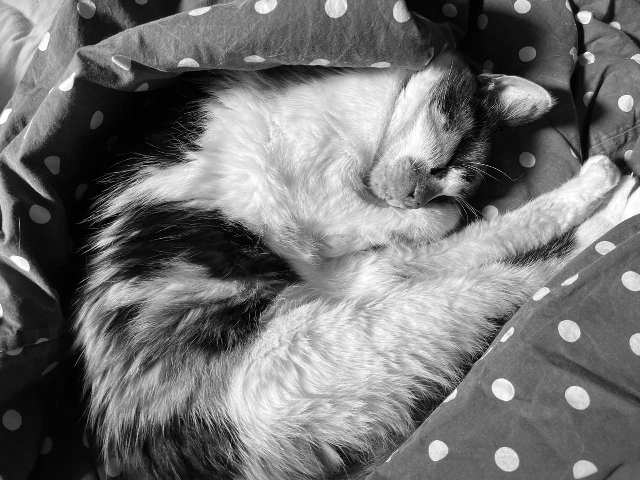
Visualize grayscale:

(bufimg/tensor->image grayscale)

Note: bufimg/tensor->image automatically handles float64→uint8 conversion and interprets single-channel tensors as grayscale images.

Histograms

A histogram shows the distribution of pixel values. It’s essential for understanding image brightness, contrast, and exposure. Peaks indicate common values; spread indicates dynamic range.

Approach 1: Overlaid BGR channels using the reshape→dataset pattern we just learned:

(-> original-tensor
    (tensor/reshape [(* height width) 3])
    tc/dataset
    (tc/rename-columns [:blue :green :red])
    (plotly/base {:=histogram-nbins 30
                  :=mark-opacity 0.5
                  :=width 800})
    (plotly/layer-histogram {:=x :red
                             :=mark-color "red"})
    (plotly/layer-histogram {:=x :blue
                             :=mark-color "blue"})
    (plotly/layer-histogram {:=x :green
                             :=mark-color "green"}))

Per-channel histograms using slice-right for clean iteration:

(kind/fragment
 (mapv (fn [color channel]
         (-> (tc/dataset {:x (dtype/as-reader channel)})
             (plotly/base {:=title color
                           :=height 200
                           :=width 800})
             (plotly/layer-histogram {:=histogram-nbins 30
                                      :=mark-color color})))
       ["blue" "green" "red"]
       (tensor/slice-right original-tensor 1)))

This approach directly iterates over sliced channels without extracting them first, combining channel names and data in a single pass.

Spatial Analysis — Edges and Gradients

We’ve explored global properties like channel means and histograms. Now let’s analyze local spatial structure by comparing neighboring pixels.

We’ll use gradient operations to measure how quickly values change across space. Gradients are fundamental to edge detection, which identifies boundaries between regions in an image.

Computing Gradients

Gradients measure how quickly pixel values change. We compute them by comparing neighboring pixels using slice offsets.

(defn gradient-x
  "Compute horizontal gradient (difference between adjacent columns).
  Takes: [H W] tensor
  Returns: [H W-1] tensor"
  [tensor-2d]
  (let [[_ w] (dtype/shape tensor-2d)]
    (dfn/- (tensor/select tensor-2d :all (range 1 w))
           (tensor/select tensor-2d :all (range 0 (dec w))))))

(defn gradient-y
  "Compute vertical gradient (difference between adjacent rows).
  Takes: [H W] tensor
  Returns: [H-1 W] tensor"
  [tensor-2d]
  (let [[h _] (dtype/shape tensor-2d)]
    (dfn/- (tensor/select tensor-2d (range 1 h) :all)
           (tensor/select tensor-2d (range 0 (dec h)) :all))))

(def gx (gradient-x grayscale))

(def gy (gradient-y grayscale))

gx

#tech.v3.tensor<float64>[960 1279]
[[ 6.000  7.000  6.000 ... -9.000 -5.000 -2.000]
 [ 5.000  6.000  5.000 ...  0.000  0.000 -1.000]
 [ 3.000  4.000  3.000 ...  5.000 -1.000 -3.000]
 ...
 [-6.000 -6.000 -6.000 ...  0.000  0.000  0.000]
 [-5.000 -3.000 -3.000 ...  0.000  0.000  0.000]
 [-5.000 -2.000 -1.000 ...  0.000  0.000  0.000]]

gy

#tech.v3.tensor<float64>[959 1280]
[[ 2.000  1.000  0.000 ...  1.000  6.000  7.000]
 [ 0.000 -2.000 -4.000 ... -5.000 -6.000 -8.000]
 [-4.000 -5.000 -7.000 ... -8.000 -12.00 -14.00]
 ...
 [ 0.000  0.000  4.000 ... -1.000 -1.000 -1.000]
 [ 4.000  5.000  8.000 ...  0.000  0.000  0.000]
 [ 6.000  6.000  7.000 ...  0.000  0.000  0.000]]

Notice: gx is one column narrower, gy is one row shorter.

Combine gradients to get edge strength: sqrt(gx² + gy²)

Why trim? gradient-x produces [H W-1] and gradient-y produces [H-1 W]. To combine them element-wise, we need matching shapes, so we trim both to [H-1 W-1].

(defn edge-magnitude
  "Compute gradient magnitude from gx and gy.
  Takes: gx [H W-1], gy [H-1 W]
  Returns: [H-1 W-1] (trimmed to common size)"
  [gx gy]
  (let [[_ w-gx] (dtype/shape gx)
        [h-gy _] (dtype/shape gy)
        ;; Trim to common dimensions: gx loses 1 row, gy loses 1 column
        gx-trimmed (tensor/select gx (range 0 h-gy) :all)
        gy-trimmed (tensor/select gy :all (range 0 w-gx))]
    (dfn/sqrt (dfn/+ (dfn/sq gx-trimmed)
                     (dfn/sq gy-trimmed)))))

(def edges (edge-magnitude gx gy))

edges

#tech.v3.tensor<float64>[959 1279]
[[6.325 7.071 6.000 ... 12.04 5.099 6.325]
 [5.000 6.325 6.403 ... 10.00 5.000 6.083]
 [5.000 6.403 7.616 ... 5.831 8.062 12.37]
 ...
 [6.000 10.00 11.70 ... 1.000 1.000 1.000]
 [7.211 7.810 10.00 ... 0.000 0.000 0.000]
 [7.810 6.708 7.616 ... 0.000 0.000 0.000]]

Visualize edges (normalize to 0-255 range):

(bufimg/tensor->image
 (-> edges
     (dfn/* (/ 255.0 (max 1.0 (dfn/reduce-max edges))))
     (dtype/elemwise-cast :uint8)))

Note: Grayscale (single-channel) tensors are rendered as grayscale images.

Sharpness Metric

Measure image sharpness by averaging edge magnitude—higher = sharper:

(defn sharpness-score
  "Compute sharpness as mean edge magnitude.
  Takes: [H W 3] BGR or [H W] grayscale tensor
  Returns: scalar (higher = sharper)"
  [img-tensor]
  (let [gray (to-grayscale img-tensor)
        gx (gradient-x gray)
        gy (gradient-y gray)
        edges (edge-magnitude gx gy)]
    (dfn/mean edges)))

(sharpness-score original-tensor)

10.654085750289296

Use case: Compare sharpness before/after blur, or rank photos by clarity.

Spatial Profiling — Row and Column Analysis

We’ve seen how to extract channels and compute global statistics. Now let’s explore row-wise and column-wise analysis using tensor/slice, tensor/transpose, and tensor/reduce-axis for spatial profiling and region detection.

Row Brightness Profile with tensor/slice

tensor/slice enables efficient iteration through rows. Let’s compute mean brightness per row to create a vertical brightness profile:

(def img-rows (tensor/slice original-tensor 1))

How many rows?

(dtype/ecount img-rows)

Compute brightness for each row:

(def row-brightness
  (mapv dfn/mean img-rows))

First 10 row brightness values:

(take 10 row-brightness)

(104.93854166666667
 105.8078125
 106.55364583333333
 106.90026041666667
 107.18020833333334
 107.37135416666666
 107.35963541666666
 107.35494791666666
 107.80833333333334
 107.74296875)

Performance note: Using tensor/slice is more efficient than manually selecting each row with (tensor/select img row-idx :all :all) in a loop, as it creates the reader once rather than performing individual selections.

Find brightest and darkest rows:

(let [brightest-idx (apply max-key #(nth row-brightness %) (range (count row-brightness)))
      darkest-idx (apply min-key #(nth row-brightness %) (range (count row-brightness)))]
  (tc/dataset
   [{:type "Brightest"
     :row-index brightest-idx
     :brightness (nth row-brightness brightest-idx)}
    {:type "Darkest"
     :row-index darkest-idx
     :brightness (nth row-brightness darkest-idx)}]))

_unnamed [2 3]:

:type	:row-index	:brightness
Brightest	577	142.36354167
Darkest	956	69.03880208

Use case: Identify horizon lines, sky regions, or exposure gradients.

Column Operations with transpose

tensor/slice only works on leftmost dimensions. For columns, we use tensor/transpose to swap dimensions:

(def img-transposed (tensor/transpose original-tensor [1 0 2]))

Shape changed from [H W C] to [W H C]:

(dtype/shape img-transposed)

[1280 960 3]

Now we can slice columns:

(def img-columns (tensor/slice img-transposed 1))

(dtype/ecount img-columns)

Compute column brightness (horizontal profile):

(def col-brightness
  (mapv dfn/mean (take 1280 img-columns)))

Visualize row vs column brightness profiles:

(-> (tc/dataset {:vertical-position (range (min 500 (count row-brightness)))
                 :row-brightness (take 500 row-brightness)})
    (plotly/base {:=title "Vertical Brightness Profile (Top 500 rows)"
                  :=x-title "Row Index"
                  :=y-title "Mean Brightness"
                  :=width 800})
    (plotly/layer-line {:=x :vertical-position
                        :=y :row-brightness
                        :=mark-color "steelblue"}))

(-> (tc/dataset {:horizontal-position (range (min 500 (count col-brightness)))
                 :col-brightness (take 500 col-brightness)})
    (plotly/base {:=title "Horizontal Brightness Profile (Left 500 columns)"
                  :=x-title "Column Index"
                  :=y-title "Mean Brightness"
                  :=width 800})
    (plotly/layer-line {:=x :horizontal-position
                        :=y :col-brightness
                        :=mark-color "coral"}))

Use case: Detect vignetting, find composition center, identify vertical features.

Efficient Aggregation with reduce-axis

For statistics without explicit iteration, use tensor/reduce-axis.

Compute row brightness using reduce-axis:

(def row-means-fast
  (-> original-tensor
      (tensor/reduce-axis dfn/mean 1 :float64) ; [H W C] → [H C]
      (tensor/reduce-axis dfn/mean 1 :float64)) ; [H C] → [H]
  )

First 10 values (compare with earlier slice-based approach):

(take 10 (dtype/as-reader row-means-fast))

(104.93854166666667
 105.8078125
 106.55364583333333
 106.90026041666665
 107.18020833333333
 107.37135416666666
 107.35963541666666
 107.35494791666667
 107.80833333333334
 107.74296875)

Why specify :float64? Without it, dtype-next might infer the output type from the input (:uint8), which would truncate decimal values from the mean operation. For example, a mean of 127.8 would become 127. Always specify the output datatype when reducing to ensure you get the precision you need.

Block-Based Region Analysis

For coarse spatial analysis, downsample into blocks and find regions of interest:

(defn downsample-blocks
  "Downsample image by averaging NxN blocks.
  Returns: [H/N W/N] tensor of block mean brightness"
  [img-tensor block-size]
  (let [[h w _] (dtype/shape img-tensor)
        new-h (quot h block-size)
        new-w (quot w block-size)]
    (tensor/compute-tensor
     [new-h new-w]
     (fn [by bx]
       (let [block (tensor/select img-tensor
                                  (range (* by block-size) (min h (* (inc by) block-size)))
                                  (range (* bx block-size) (min w (* (inc bx) block-size)))
                                  :all)]
         (dfn/mean block)))
     :float32)))

(def brightness-map (downsample-blocks original-tensor 20))

Brightness map shape:

(dtype/shape brightness-map)

[48 64]

[48 64] for 960/20 × 1280/20

Find brightest and darkest blocks:

(defn find-block-extremes
  "Find coordinates of brightest and darkest blocks in a 2D tensor."
  [tensor-2d]
  (let [flat (dtype/as-reader (tensor/reshape tensor-2d [(dtype/ecount tensor-2d)]))
        [h w] (dtype/shape tensor-2d)
        max-idx (apply max-key #(flat %) (range (dtype/ecount flat)))
        min-idx (apply min-key #(flat %) (range (dtype/ecount flat)))]
    {:brightest {:block-y (quot max-idx w)
                 :block-x (rem max-idx w)
                 :value (flat max-idx)}
     :darkest {:block-y (quot min-idx w)
               :block-x (rem min-idx w)
               :value (flat min-idx)}}))

(find-block-extremes brightness-map)

{:brightest {:block-y 20, :block-x 63, :value 247.27},
 :darkest {:block-y 12, :block-x 13, :value 2.08}}

Use case: Quick region-of-interest detection, composition analysis, exposure mapping.

Enhancement Pipeline

We’ve explored analyzing image properties—now let’s actively transform them. With analysis tools in place, we’ll build functions that improve images through white balance and contrast adjustment. Each transformation is composable and verifiable through numeric properties we can check in the REPL.

Auto White Balance

White balance adjusts colors to appear neutral under different lighting conditions. We scale BGR channels to have equal means, removing color casts.

(defn auto-white-balance
  "Scale BGR channels to have equal means.
  Takes: [H W 3] uint8 BGR tensor
  Returns: [H W 3] uint8 BGR tensor"
  [img-tensor]
  (let [;; Compute channel means using reduce-axis
        ;; First reduce: [H W 3] → [W 3] (collapse height, axis 0)
        ;; Second reduce: [W 3] → [3] (collapse width, now axis 0 after shape change)
        channel-means (-> img-tensor
                          (tensor/reduce-axis dfn/mean 0) ; [H W 3] → [W 3]
                          (tensor/reduce-axis dfn/mean 0)) ; [W 3] → [3]

        ;; Target: maximum of the three means
        target-mean (dfn/reduce-max channel-means)

        ;; Compute scale factors for each channel [3]
        scale-factors (dfn// target-mean (dfn/max 1.0 channel-means))

        [h w c] (dtype/shape img-tensor)

        ;; Scale each channel (vectorized operations per channel)
        scaled-channels (mapv (fn [ch]
                                (let [channel (tensor/select img-tensor :all :all ch)
                                      scale (scale-factors ch)]
                                  (dtype/elemwise-cast
                                   (dfn/min 255 (dfn/* channel scale))
                                   :uint8)))
                              (range c))]

    ;; Reassemble channels
    (tensor/compute-tensor
     [h w c]
     (fn [y x ch]
       ((nth scaled-channels ch) y x))
     :uint8)))

(kind/table
 [[:original
   :white-balanced]
  [original-img
   (-> original-tensor
       auto-white-balance
       bufimg/tensor->image)]])

original	white-balanced

BGR tensor → BGR image

Note: Our BGR tensor flows seamlessly to BGR BufferedImage.

Contrast Enhancement

Contrast enhancement amplifies the difference between light and dark regions. We amplify each pixel’s deviation from the mean, making bright pixels brighter and dark pixels darker.

(defn enhance-contrast
  "Increase image contrast by amplifying deviation from mean.
  Takes: [H W 3] uint8 BGR tensor, factor (> 1 increases, < 1 decreases)
  Returns: [H W 3] uint8 BGR tensor"
  [img-tensor factor]
  (let [[h w c] (dtype/shape img-tensor)

        ;; Process each channel independently
        enhanced-channels (mapv (fn [ch]
                                  (let [channel (tensor/select img-tensor :all :all ch)
                                        ch-mean (dfn/mean channel)]
                                    ;; Apply contrast: mean + factor * (value - mean)
                                    (dtype/elemwise-cast
                                     (dfn/min 255
                                              (dfn/max 0
                                                       (dfn/+ ch-mean
                                                              (dfn/* (dfn/- channel ch-mean) factor))))
                                     :uint8)))
                                (range c))]

    ;; Reassemble channels
    (tensor/compute-tensor
     [h w c]
     (fn [y x ch]
       ((nth enhanced-channels ch) y x))
     :uint8)))

(def contrasted (enhance-contrast original-tensor 1.5))

(kind/table
 [[:original
   :contrast-1.5
   :contrast-3]
  [original-img
   (-> original-tensor
       (enhance-contrast 1.5)
       bufimg/tensor->image) ; BGR → BGR
   (-> original-tensor
       (enhance-contrast 3)
       bufimg/tensor->image)]])

original	contrast-1.5	contrast-3

Accessibility — Color Blindness Simulation

Beyond enhancement, images need to be accessible. Let’s simulate how images appear to people with different types of color vision deficiency.

This demonstrates dtype-next’s linear algebra capabilities (applying 3×3 matrices to BGR channels) with practical real-world applications.

Apply 3×3 transformation matrices to simulate different types of color vision deficiency.

Color Blindness Matrices

These matrices simulate color blindness (color vision deficiency). Different types affect perception of red, green, or blue:

(def color-blindness-matrices
  "Color blindness simulation matrices.
  Each matrix is 3×3 with columns in BGR order: [B G R]
  Matrices adapted from standard RGB formulas, reordered for BGR."
  {:protanopia [[0.000 0.433 0.567] ; Red-blind (BGR columns)
                [0.000 0.442 0.558]
                [0.758 0.242 0.000]]

   :deuteranopia [[0.000 0.375 0.625] ; Green-blind (BGR columns)
                  [0.000 0.300 0.700]
                  [0.700 0.300 0.000]]

   :tritanopia [[0.000 0.050 0.950] ; Blue-blind (BGR columns)
                [0.567 0.433 0.000]
                [0.525 0.475 0.000]]})

Applying Matrix Transformations

Extract BGR channels, apply linear combinations, reassemble:

(defn apply-color-matrix
  "Apply 3×3 transformation matrix to BGR channels.
  Takes: [H W 3] BGR tensor, 3×3 matrix [[b0 g0 r0] [b1 g1 r1] [b2 g2 r2]]
  Returns: [H W 3] uint8 BGR tensor
  Formula: new_b = b0*B + g0*G + r0*R, etc.
  
  Note: Matrix coefficients correspond to BGR order (channel 0=B, 1=G, 2=R)"
  [img-tensor matrix]
  (let [b (tensor/select img-tensor :all :all 0) ; Blue channel
        g (tensor/select img-tensor :all :all 1) ; Green channel
        r (tensor/select img-tensor :all :all 2) ; Red channel

        [[b0 g0 r0]
         [b1 g1 r1]
         [b2 g2 r2]] matrix

        ;; Apply transformation (BGR order)
        new-b (dfn/+ (dfn/+ (dfn/* b b0) (dfn/* g g0)) (dfn/* r r0))
        new-g (dfn/+ (dfn/+ (dfn/* b b1) (dfn/* g g1)) (dfn/* r r1))
        new-r (dfn/+ (dfn/+ (dfn/* b b2) (dfn/* g g2)) (dfn/* r r2))

        ;; Clamp and cast
        clamp-cast (fn [ch]
                     (dtype/elemwise-cast
                      (dfn/min 255 (dfn/max 0 ch))
                      :uint8))

        new-b-clamped (clamp-cast new-b)
        new-g-clamped (clamp-cast new-g)
        new-r-clamped (clamp-cast new-r)

        [h w _] (dtype/shape img-tensor)]
    (tensor/compute-tensor
     [h w 3]
     (fn [y x c]
       (case c
         0 (new-b-clamped y x) ; Blue channel 0
         1 (new-g-clamped y x) ; Green channel 1
         2 (new-r-clamped y x))) ; Red channel 2
     :uint8)))

(defn simulate-color-blindness
  "Simulate color vision deficiency.
  Takes: [H W 3] tensor, blindness-type (:protanopia | :deuteranopia | :tritanopia)
  Returns: [H W 3] uint8 tensor"
  [img-tensor blindness-type]
  (apply-color-matrix img-tensor
                      (get color-blindness-matrices blindness-type)))

Simulations

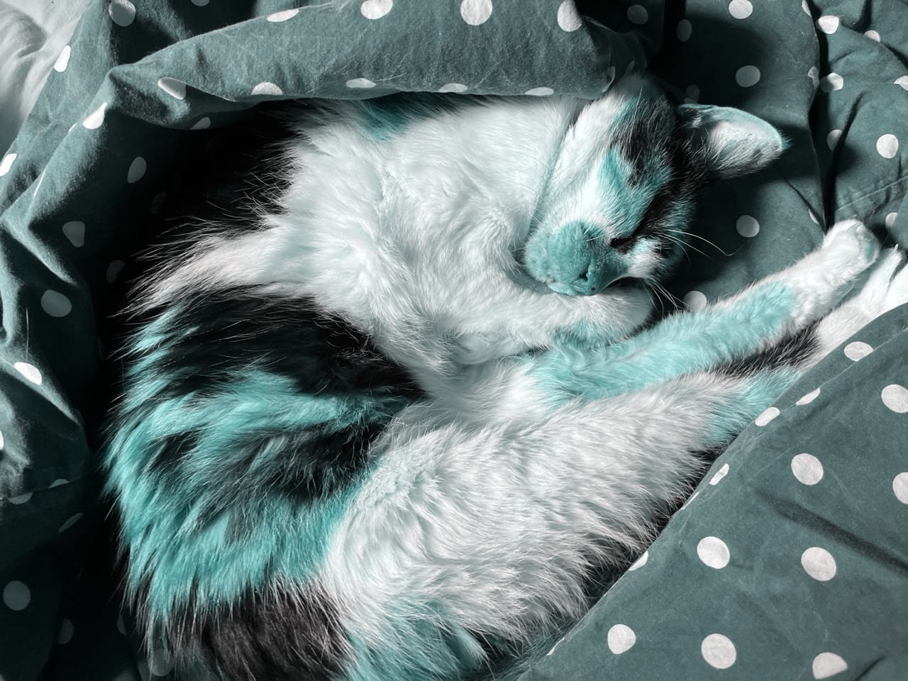
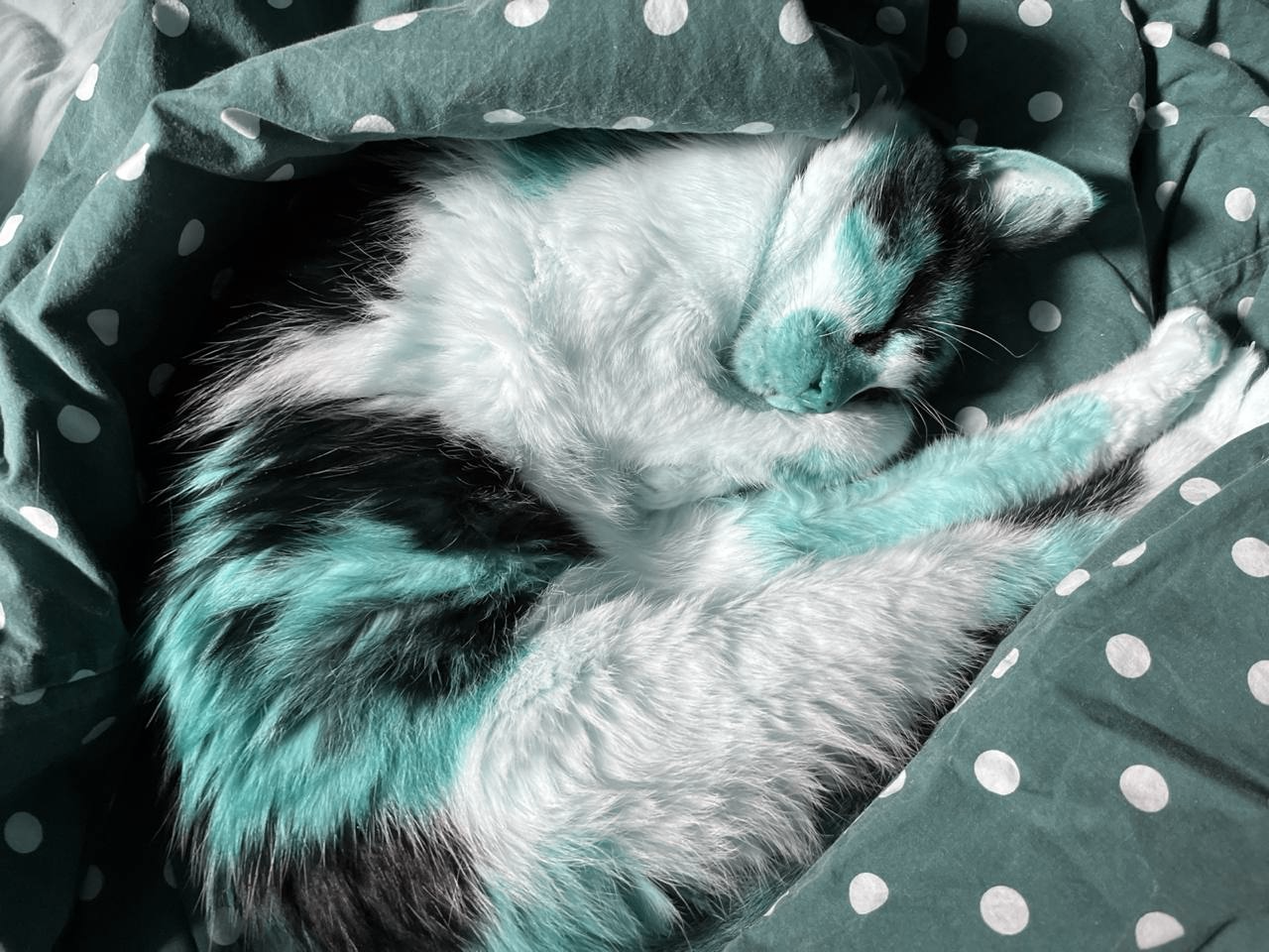
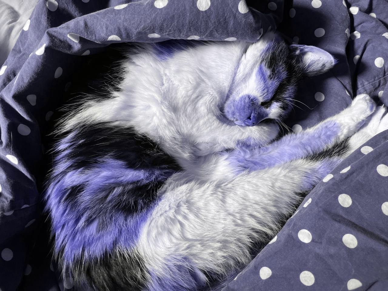
(kind/table
 [[:normal :protanopia :deuteranopia :tritanopia]
  [(bufimg/tensor->image original-tensor)
   (bufimg/tensor->image (simulate-color-blindness original-tensor :protanopia))
   (bufimg/tensor->image (simulate-color-blindness original-tensor :deuteranopia))
   (bufimg/tensor->image (simulate-color-blindness original-tensor :tritanopia))]])

normal	protanopia	deuteranopia	tritanopia

All color blindness transformations maintain BGR order throughout.

Convolution & Filtering

So far we’ve used simple element-wise operations and direct pixel comparisons. Now let’s explore convolution, the fundamental operation behind blur, sharpen, and edge detection.

What we’ll learn:

How convolution works (sliding kernels over images)
Building a 2D convolution function for learning and non-separable filters
Separable filters—the standard approach for Gaussian blur
Practical applications: box blur, Gaussian blur, sharpening, edge detection

Understanding Convolution

Convolution is a fundamental operation in image processing. A kernel (or filter) is a small matrix that slides over the image. At each position, we multiply kernel values by corresponding pixel values and sum the result.

Let’s see this with a simple example: box blur.

Box Blur Example

Box blur averages all pixels in a neighborhood. A 3×3 box blur kernel weights all 9 pixels equally:

(defn box-blur-kernel
  "Create NxN box blur kernel (uniform averaging).
  Takes: n (kernel size)
  Returns: [n n] float32 tensor"
  [n]
  (let [weight (/ 1.0 (* n n))]
    (tensor/compute-tensor
     [n n]
     (fn [_ _] weight)
     :float32)))

(def kernel-3x3 (box-blur-kernel 3))

kernel-3x3

[#tech.v3.tensor<float32>[3]
[0.1111 0.1111 0.1111] #tech.v3.tensor<float32>[3]
[0.1111 0.1111 0.1111] #tech.v3.tensor<float32>[3]
[0.1111 0.1111 0.1111]]

This kernel says: “Replace each pixel with the average of itself and its 8 neighbors.” To apply this kernel across the entire image, we need a convolution function.

Building a 2D Convolution Function

We’ll implement convolve-2d to understand the mechanics. This function is useful for:

Learning: See exactly how convolution works
Non-separable filters: Some kernels (like Sobel) can’t be separated into 1D operations

For separable filters like Gaussian blur, we’ll use a more efficient approach (shown next).

(defn convolve-2d
  "Apply 2D convolution to grayscale image [H W].
  kernel: [kh kw] float tensor
  edge-mode: :zero (default) or :reflect
  Returns [H W] float32 tensor.
  
  This implementation prioritizes clarity over performance to demonstrate
  tensor operations and convolution mechanics. It explicitly shows:

  - Sliding window iteration with loop/recur
  - Bounds checking and edge handling
  - Element-wise kernel multiplication
  
  This function is useful for learning and for non-separable kernels.
  For separable filters like Gaussian blur, see gaussian-blur-separable below."
  ([img-2d kernel] (convolve-2d img-2d kernel :zero))
  ([img-2d kernel edge-mode]
   (let [[h w] (dtype/shape img-2d)
         [kh kw] (dtype/shape kernel)
         pad-h (quot kh 2)
         pad-w (quot kw 2)

         ;; Helper to get pixel value with edge handling
         get-pixel (case edge-mode
                     :zero (fn [y x]
                             (if (and (>= y 0) (< y h)
                                      (>= x 0) (< x w))
                               (img-2d y x)
                               0.0))
                     :reflect (fn [y x]
                                (let [ry (cond
                                           (< y 0) (- y)
                                           (>= y h) (- h (- y h) 2)
                                           :else y)
                                      rx (cond
                                           (< x 0) (- x)
                                           (>= x w) (- w (- x w) 2)
                                           :else x)]
                                  (img-2d (max 0 (min (dec h) ry))
                                          (max 0 (min (dec w) rx))))))]
     (tensor/compute-tensor
      [h w]
      (fn [y x]
        ;; Sum weighted pixel values in kernel neighborhood
        (loop [ky 0
               kx 0
               sum 0.0]
          (if (>= ky kh)
            sum
            (let [img-y (+ y ky (- pad-h))
                  img-x (+ x kx (- pad-w))
                  pixel-val (get-pixel img-y img-x)
                  new-sum (+ sum (* (kernel ky kx) pixel-val))
                  [next-ky next-kx] (if (>= (inc kx) kw)
                                      [(inc ky) 0]
                                      [ky (inc kx)])]
              (recur next-ky next-kx new-sum)))))
      :float32))))

Separable Filters: The Recommended Approach

Many important filters are separable—they can be decomposed into two 1D operations instead of one 2D operation. This is the standard approach for filters like Gaussian blur, not an optimization.

How it works: Instead of applying a k×k kernel to each pixel, we: 1. Apply a 1D kernel horizontally (blur each row) 2. Apply a 1D kernel vertically (blur each column)

Computational advantage:

2D convolution with k×k kernel: O(k²) operations per pixel
Separable approach: O(k) operations per pixel (k/2 horizontal + k/2 vertical)
For a 7×7 kernel: 49 vs 7 operations per pixel (~7× reduction)

Where:

k = kernel size (e.g., 7 for a 7×7 kernel)
N×M = image dimensions (height × width)
Total work for image: O(N×M×k²) vs O(N×M×k)

Additional optimizations: Library functions like convolve/gaussian1d may use FFT (Fast Fourier Transform) for very large kernels or data, which can be even faster: O(N×M×log(N×M)) regardless of kernel size. This happens automatically based on data size.

The convolve Namespace

(require '[tech.v3.datatype.convolve :as convolve])

The tech.v3.datatype.convolve namespace provides optimized 1D convolution operations:

convolve/gaussian1d — 1D Gaussian filter with automatic kernel generation
convolve/convolve1d — General 1D convolution
convolve/gauss-kernel-1d — Create 1D Gaussian kernels

These functions support edge-handling strategies (:zero, :clamp, :reflect, :wrap) and may use FFT optimization automatically for large data.

(defn gaussian-blur-separable
  "Apply Gaussian blur using separable 1D convolutions.
  Takes: [H W] grayscale tensor, sigma (standard deviation)
  Returns: [H W] float64 tensor
  
  This is the recommended approach for Gaussian blur.
  Applies horizontal blur to each row, then vertical blur to each column."
  [img-2d sigma]
  (let [[h w] (dtype/shape img-2d)

        ;; Step 1: Blur each row horizontally
        ;; tensor/slice gives us a reader of rows (zero-copy)
        rows (tensor/slice img-2d 1)

        ;; dtype/emap applies gaussian1d to each row (lazy)
        rows-blurred (dtype/emap
                      (fn [row]
                        (convolve/gaussian1d row sigma {:mode :same :edge-mode :reflect}))
                      :object
                      rows)

        ;; Concatenate blurred rows into single buffer, then reshape to [h w]
        horizontal-blurred (tensor/reshape
                            (dtype/concat-buffers :float64 rows-blurred)
                            [h w])

        ;; Step 2: Blur each column vertically
        ;; tensor/slice-right gives us a reader of columns (zero-copy)
        cols (tensor/slice-right horizontal-blurred 1)

        cols-blurred (dtype/emap
                      (fn [col]
                        (convolve/gaussian1d col sigma {:mode :same :edge-mode :reflect}))
                      :object
                      cols)]

    ;; Reassemble columns (requires transposition, so use compute-tensor)
    (tensor/compute-tensor
     [h w]
     (fn [y x]
       ((nth cols-blurred x) y))
     :float64)))

Key dtype-next patterns in this implementation:

tensor/slice and tensor/slice-right — Zero-copy readers of rows/columns
dtype/emap — Lazy transformation over readers (more efficient than mapv)
dtype/concat-buffers — Efficiently concatenate buffers for reassembly
tensor/reshape — Zero-copy view with different shape
tensor/compute-tensor — Used when data needs reordering (columns → rows)

The horizontal pass uses concat-buffers + reshape (fast, sequential data). The vertical pass uses compute-tensor (necessary for transposition).

The convolve/gaussian1d function handles kernel generation, edge modes (:reflect, :wrap, :zero), and may use FFT optimization automatically for large data.

With separable filters understood, let’s apply convolution to practical filtering tasks.

Applying Box Blur

Now we can apply our 3×3 box blur kernel using convolve-2d:

(def blurred-gray (convolve-2d grayscale kernel-3x3))

Compare original vs blurred:

(kind/table
 [[:original :box-blur-3x3]
  [(bufimg/tensor->image grayscale)
   (bufimg/tensor->image (dtype/elemwise-cast blurred-gray :uint8))]])

original	box-blur-3x3

Box blur creates a simple averaging effect. Grayscale tensors (2D) are automatically rendered as grayscale images.

Gaussian Blur (Separable)

Gaussian blur weights center pixels more heavily than edge pixels based on the Gaussian (normal) distribution, producing smooth, natural-looking blur without artifacts.

We use gaussian-blur-separable (the recommended approach):

(def gaussian-blurred-1 (gaussian-blur-separable grayscale 1.0))

(def gaussian-blurred-1-5 (gaussian-blur-separable grayscale 1.5))

Compare blur strengths—notice how Gaussian blur is smoother than box blur:

(kind/table
 [[:original :box-blur-3x3 :gaussian-sigma-1.0 :gaussian-sigma-1.5]
  [(bufimg/tensor->image grayscale)
   (bufimg/tensor->image (dtype/elemwise-cast blurred-gray :uint8))
   (bufimg/tensor->image gaussian-blurred-1)
   (bufimg/tensor->image gaussian-blurred-1-5)]])

original	box-blur-3x3	gaussian-sigma-1.0	gaussian-sigma-1.5

Sharpening (Unsharp Masking)

Unsharp masking sharpens images by enhancing edges. We subtract a blurred version from the original to extract high-frequency details, then add them back amplified:

Formula: sharpened = original + strength × (original - blur)

(defn sharpen
  "Sharpen image using unsharp mask.
  Takes: [H W] grayscale tensor, strength (0.5-2.0 typical)
  Returns: [H W] float32 tensor"
  [img-2d strength]
  (let [blurred (convolve-2d img-2d (box-blur-kernel 3))
        detail (dfn/- img-2d blurred)]
    (-> (dfn/+ img-2d (dfn/* detail strength))
        (dfn/max 0)
        (dfn/min 255))))

(def sharpened-gray (sharpen grayscale 1.5))

Compare original vs sharpened:

(kind/table
 [[:original :sharpened]
  [(bufimg/tensor->image grayscale)
   (bufimg/tensor->image (dtype/elemwise-cast sharpened-gray :uint8))]])

original	sharpened

Quantifying Sharpness

We can measure the effect of each filter by computing mean edge magnitude. Higher values = sharper images, lower values = blurrier:

(-> {:original grayscale
     :box-blur-3x3 blurred-gray
     :gaussian-sigma-1.0 gaussian-blurred-1
     :gaussian-sigma-1.5 gaussian-blurred-1-5
     :sharpened sharpened-gray}
    (update-vals
     (fn [t]
       (dfn/mean (edge-magnitude
                  (gradient-x t)
                  (gradient-y t)))))
    tc/dataset)

_unnamed [1 5]:

:original	:box-blur-3x3	:gaussian-sigma-1.0	:gaussian-sigma-1.5	:sharpened
10.65408575	5.89871815	5.25806474	3.95598023	20.40900352

As expected: sharpening increases edge magnitude, blurring decreases it.

Sobel Edge Detection

The Sobel operator is a classic edge detection method that uses specialized kernels to compute gradients in X and Y directions. It’s more robust to noise than simple finite differences.

Sobel kernels detect edges in X and Y directions:

(def sobel-x-kernel
  (tensor/compute-tensor
   [3 3]
   (fn [y x]
     (case [y x]
       [0 0] -1.0, [0 1] 0.0, [0 2] 1.0
       [1 0] -2.0, [1 1] 0.0, [1 2] 2.0
       [2 0] -1.0, [2 1] 0.0, [2 2] 1.0))
   :float32))

(def sobel-y-kernel
  (tensor/compute-tensor
   [3 3]
   (fn [y x]
     (case [y x]
       [0 0] -1.0, [0 1] -2.0, [0 2] -1.0
       [1 0] 0.0, [1 1] 0.0, [1 2] 0.0
       [2 0] 1.0, [2 1] 2.0, [2 2] 1.0))
   :float32))

Apply Sobel filters:

(def sobel-x (convolve-2d grayscale sobel-x-kernel))

(def sobel-y (convolve-2d grayscale sobel-y-kernel))

Compute edge magnitude:

(def sobel-edges (dfn/sqrt (dfn/+ (dfn/sq sobel-x) (dfn/sq sobel-y))))

Visualize Sobel edges:

(bufimg/tensor->image
 (-> sobel-edges
     (dfn/* (/ 255.0 (max 1.0 (dfn/reduce-max sobel-edges))))
     (dtype/elemwise-cast :uint8)))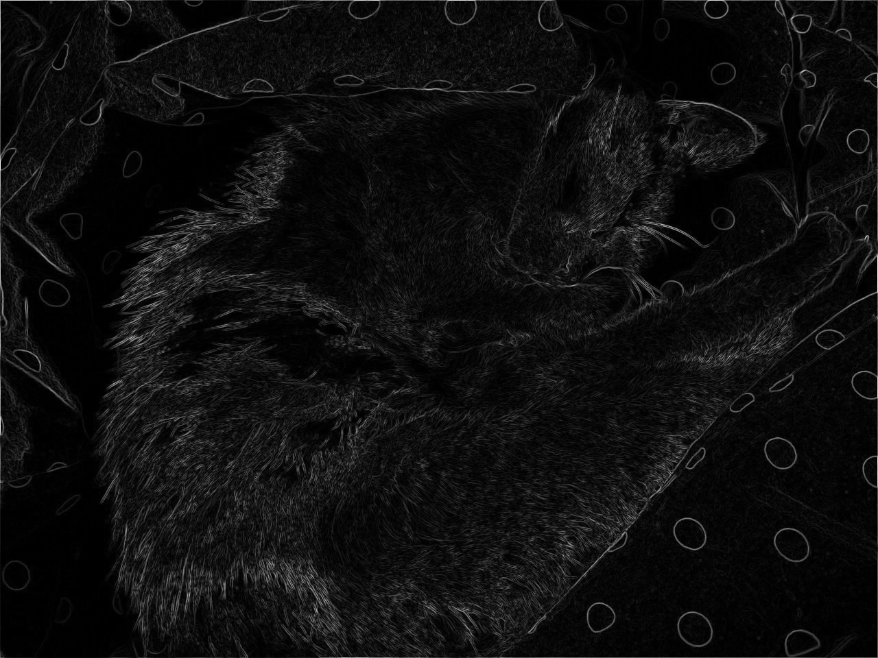

Single-channel tensors display as grayscale images.

Comparison: Simple gradient (from Spatial Analysis section) vs Sobel

{:simple-mean (dfn/mean edges) ; reuse edges computed earlier
 :sobel-mean (dfn/mean sobel-edges)
 :sobel-smoother? true}

{:simple-mean 10.654085750289296,
 :sobel-mean 59.98076450272415,
 :sobel-smoother? true}

Sobel produces smoother, more robust edge detection.

Downsampling & Multi-Scale Processing

Finally, let’s explore working with images at multiple scales. Downsampling reduces resolution for faster processing or multi-scale analysis (like detecting features at different sizes).

We’ll compare downsampling strategies and build image pyramids, demonstrating tensor/select with stride patterns and aggregation techniques.

Downsampling by 2×

Downsampling (decimation) reduces image resolution by discarding pixels. We select every other pixel in each dimension, creating a half-size image.

(defn downsample-2x
  "Downsample by selecting every other pixel.
  Takes: [H W] tensor
  Returns: [H/2 W/2] tensor"
  [img-2d]
  (let [[h w] (dtype/shape img-2d)]
    (tensor/select img-2d (range 0 h 2) (range 0 w 2))))

(def downsampled-gray (downsample-2x grayscale))

(tc/dataset {:metric ["Original height" "Original width"
                      "Downsampled height" "Downsampled width"]
             :value (let [[oh ow] (dtype/shape grayscale)
                          [dh dw] (dtype/shape downsampled-gray)]
                      [oh ow dh dw])})

_unnamed [4 2]:

:metric	:value
Original height	960
Original width	1280
Downsampled height	480
Downsampled width	640

Visualize original vs downsampled:

(kind/table
 [[:original :downsampled-2x]
  [(bufimg/tensor->image grayscale)
   (bufimg/tensor->image downsampled-gray)]])

original	downsampled-2x

Both grayscale tensors render as grayscale images.

Image Pyramid

An image pyramid contains the same image at multiple scales. This is essential for multi-scale analysis, feature detection at different sizes, and efficient image processing algorithms.

(defn build-pyramid
  "Build image pyramid with multiple scales.
  Takes: [H W] tensor, levels (number of scales)
  Returns: vector of tensors [[H W] [H/2 W/2] [H/4 W/4] ...]"
  [img-2d levels]
  (loop [pyramid [img-2d]
         current img-2d
         level 1]
    (if (>= level levels)
      pyramid
      (let [next-level (downsample-2x current)]
        (recur (conj pyramid next-level)
               next-level
               (inc level))))))

(def gray-pyramid (build-pyramid grayscale 4))

Inspect pyramid shapes:

(tc/dataset {:level (range (count gray-pyramid))
             :height (mapv #(first (dtype/shape %)) gray-pyramid)
             :width (mapv #(second (dtype/shape %)) gray-pyramid)})

_unnamed [4 3]:

:level	:height	:width
0	960	1280
1	480	640
2	240	320
3	120	160

Visualize each level:

(kind/fragment
 (mapv bufimg/tensor->image gray-pyramid))

Each grayscale tensor at different scales renders as a grayscale image.

Use case: Multi-scale edge detection for finding features at different sizes.

Block Average Downsampling

Instead of selecting pixels, we can average blocks for smoother downsampling:

(defn downsample-avg
  "Downsample by averaging blocks.
  Takes: [H W] tensor, factor (downsampling factor)
  Returns: [H/factor W/factor] float32 tensor"
  [img-2d factor]
  (let [[h w] (dtype/shape img-2d)
        new-h (quot h factor)
        new-w (quot w factor)]
    (tensor/compute-tensor
     [new-h new-w]
     (fn [y x]
       (let [block (tensor/select img-2d
                                  (range (* y factor) (* (inc y) factor))
                                  (range (* x factor) (* (inc x) factor)))]
         (dfn/mean block)))
     :float32)))

(def avg-downsampled (downsample-avg grayscale 2))

Compare simple vs average downsampling:

(kind/table
 [[:select-every-2nd :average-blocks]
  [(bufimg/tensor->image downsampled-gray)
   (bufimg/tensor->image avg-downsampled)]])

select-every-2nd	average-blocks

Both are grayscale. tensor->image handles float32 → uint8 conversion automatically.

Average downsampling produces smoother results with less aliasing.

Verification: Both produce same shape, but averaging reduces noise

(tc/dataset {:method ["Select every 2nd" "Average blocks"]
             :height (mapv #(first (dtype/shape %)) [downsampled-gray avg-downsampled])
             :width (mapv #(second (dtype/shape %)) [downsampled-gray avg-downsampled])
             :mean (mapv dfn/mean [downsampled-gray avg-downsampled])})

_unnamed [2 4]:

:method	:height	:width	:mean
Select every 2nd	480	640	115.39179457
Average blocks	480	640	115.37941120

Conclusion: The dtype-next Pattern

We started with a simple question: Why use dtype-next for image processing?

Through building a complete analysis toolkit—from channel statistics to edge detection to convolution—we’ve seen the answer in action:

Efficient typed arrays replace boxed sequences, saving memory and enabling SIMD
Zero-copy views let us slice and transform without allocation overhead
Functional composition keeps operations pure and composable
Immediate visual feedback makes abstract tensor operations concrete and verifiable

Images provided the perfect learning vehicle: every transformation has visible results we can inspect in the REPL. The patterns we’ve practiced transfer directly to any domain requiring efficient numerical computing.

Key Patterns

Zero-copy views — tensor/select creates views without copying data
Reduction operations — dfn/mean, dfn/standard-deviation, etc.
Element-wise ops — dfn/+, dfn/*, dfn/sqrt work across entire tensors
Type discipline — upcast → compute → clamp → downcast for precision control
Functional composition — pure functions composed with -> and function composition
Objective verification — numeric properties that can be checked in REPL

API Coverage

Here are the key dtype-next functions we used throughout this tutorial:

dtype namespace (tech.v3.datatype):

dtype/shape — Inspect tensor dimensions
dtype/elemwise-datatype — Check element type
dtype/elemwise-cast — Convert between types
dtype/ecount — Total element count
dtype/as-reader — Convert to readable sequence
Readers act as functions: (reader idx) instead of (dtype/get-value reader idx)

tensor namespace (tech.v3.tensor):

tensor/compute-tensor — Functionally construct tensors
tensor/select — Extract slices, channels (zero-copy)
Tensors act as functions: (tensor y x) instead of (tensor/mget tensor y x)
tensor/reshape — Reinterpret tensor shape (zero-copy)
tensor/reduce-axis — Reduce along specific dimension

dfn namespace (tech.v3.datatype.functional):

dfn/+, dfn/-, dfn/*, dfn// — Element-wise arithmetic
dfn/mean, dfn/standard-deviation — Statistics
dfn/reduce-min, dfn/reduce-max — Range finding
dfn/sqrt, dfn/sq — Mathematical operations
dfn/min, dfn/max — Clamping
dfn/sum — Summation

bufimg namespace (tech.v3.libs.buffered-image):

bufimg/load — Load image file
bufimg/as-ubyte-tensor — BufferedImage → tensor
bufimg/tensor->image — tensor → BufferedImage
bufimg/image-type — Check image format

What Makes This Functional?

Pure functions — all transformations return new values
Immutable views — original data never changes
Composition — operations chain naturally
Lazy evaluation — computations deferred until needed
No mutation — even tensor/compute-tensor builds new structures

Beyond Images: dtype-next in Other Domains

The tensor patterns we’ve explored transfer directly to other use cases:

Time series analysis: 1D or 2D tensors for signals, windowing operations for feature extraction, functional ops for filtering and aggregation.

Scientific computing: Multi-dimensional numerical arrays, zero-copy slicing for memory efficiency, type discipline for numerical precision.

Machine learning prep: Batch processing, normalization pipelines, data augmentation—all using the same functional patterns.

Signal processing: Audio (1D), video (4D: time×height×width×channels), sensor arrays—dtype-next handles arbitrary dimensionality.

dtype-next also provides:

Native interop: Zero-copy integration with native libraries (OpenCV, Numpy, etc.)
Dataset tools: Rich tech.ml.dataset integration for tabular workflows
Performance: SIMD-optimized operations, parallel processing support
Flexibility: Custom buffer implementations, extensible type system

Resources

Questions, corrections, or ideas? Open an issue on the Clojure Civitas repository.

source: src/dtype_next/image_processing_with_tensors.clj