Rolling Regressions in Clojure for Real-Time Alpha and Beta Monitoring
1. Abstract
This blog post presents a functional, reproducible implementation of rolling regression in Clojure to estimate time-varying alpha(α) and beta(β) for student-managed portfolios at the Centre for Investment Management (CIM), The University of Hong Kong. Unlike traditional CAPM tests based on passive index data, our analysis uses actual(synthetic) trades executed by junior portfolio managers- undergraduate students who manage simulated equity portfolios over multiple semesters.
2. Data and Methodology
2.1. Data Sources
We use hypothetical trade data from student portfolio managers at the Centre for Investment Management, including:
● Trade dates, tickers, shares, prices
● Portfolio valuations over time(monthly rebalancing)
● Cash flows and position weights
● Returns are computed at the portfolio level, aggregated monthly from individual holdings.
● Benchmark: S&P 500 total return index
● Excess returns are calculated for both portfolios and the market.
● The risk free rate is omitted from analysis for ease of understanding concepts since it does not affect the final results presented in this proposal
2.2. Rolling Market Model
For each student portfolio, we estimate the CAPM regression over a rolling 12- or 24-month window:
Using ordinary least squares(OLS), we obtain a time series of:
● Alpha(α): time-varying abnormal return(skill or luck?)
● Beta(β): evolving sensitivity to market movements(risk awareness?)
● Windows slide forward monthly, producing a dynamic view of performance.
3. Implementation in Clojure
The full analysis pipeline is implemented in Clojure, designed for clarity, reuse, and integration into teaching workflows. Below are some core libraries that were used in the project.
Core Libraries
● generateme/fastmath: for OLS regression and statistical operations
● scicloj/tablecloth: for data preparation and transformation
● clj-python/libpython-clj: to fetch price data using the yfinance library in Python
● org.clojure/data.csv: for inputting securities for analysis
● org.clojure/clojure.data.json: to parse JSON strings
Code Preview
The below function uses a simple Python script (with the help of clj-python to integrate Python with Clojure) to fetch open and closing prices for NVIDIA stocks and the S&P 500 Index from Yahoo Finance.
(def get-python-data
  (py/run-simple-string
       "from datetime import datetime, timedelta
        import yfinance as yf

        # Both are already in USD

        nvidia_data = yf.download('NVDA', start='2022-09-01', end='2025-09-01')
        snp_data = stock_data = yf.download('^GSPC', start='2022-09-01', end='2025-09-01')

        nvidia_data.reset_index(inplace=True)
        snp_data.reset_index(inplace=True)

        nvidia_data['Date'] = nvidia_data['Date'].dt.strftime('%Y-%m-%d')
        snp_data['Date'] = snp_data['Date'].dt.strftime('%Y-%m-%d')

        stock_data = nvidia_data[['Date', 'Open', 'Close']].to_json(orient = 'values')
        market_data = snp_data[['Date', 'Open', 'Close']].to_json(orient = 'values')"))
We can then obtain data as follows:
(def stock-data (json/read-str (:stock_data (:globals get-python-data))))stock-data[["2022-09-01" 14.1885330018 13.9169254303]
["2022-09-02" 14.0796907453 13.6273431778]
["2022-09-06" 13.7112209556 13.4456043243]
["2022-09-07" 13.5474882899 13.6983156204]
["2022-09-08" 13.4436062056 13.9739990234]
["2022-09-09" 14.1408088859 14.3705463409]
["2022-09-12" 14.3525677558 14.4884119034]
["2022-09-13" 13.7862151343 13.1159820557]
["2022-09-14" 13.2388419174 13.1129865646]
["2022-09-15" 13.0001152655 12.9142131805]
["2022-09-16" 12.7274264037 13.1829051971]
["2022-09-19" 12.9971186755 13.3666954041]
["2022-09-20" 13.1998874975 13.1609315872]
["2022-09-21" 13.1978908111 13.2458353043]
["2022-09-22" 13.0550504041 12.5466327667]
["2022-09-23" 12.4057942741 12.5016841888]
["2022-09-26" 12.4767137378 12.2140140533]
["2022-09-27" 12.4926960686 12.3988037109]
["2022-09-28" 12.3958072082 12.7214345932]
["2022-09-29" 12.4337640638 12.2060251236]
["2022-09-30" 12.0731767255 12.1251173019]](def market-data (json/read-str (:market_data (:globals get-python-data))))market-data[["2022-09-01" 3936.7299804688 3966.8500976562]
["2022-09-02" 3994.6599121094 3924.2600097656]
["2022-09-06" 3930.8898925781 3908.1899414062]
["2022-09-07" 3909.4299316406 3979.8701171875]
["2022-09-08" 3959.9399414062 4006.1799316406]
["2022-09-09" 4022.9399414062 4067.3601074219]
["2022-09-12" 4083.669921875 4110.41015625]
["2022-09-13" 4037.1201171875 3932.6899414062]
["2022-09-14" 3940.7299804688 3946.0100097656]
["2022-09-15" 3932.4099121094 3901.3500976562]
["2022-09-16" 3880.9499511719 3873.330078125]
["2022-09-19" 3849.9099121094 3899.8898925781]
["2022-09-20" 3875.2299804688 3855.9299316406]
["2022-09-21" 3871.3999023438 3789.9299316406]
["2022-09-22" 3782.3601074219 3757.9899902344]
["2022-09-23" 3727.1398925781 3693.2299804688]
["2022-09-26" 3682.7199707031 3655.0400390625]
["2022-09-27" 3686.4399414062 3647.2900390625]
["2022-09-28" 3651.9399414062 3719.0400390625]
["2022-09-29" 3687.0100097656 3640.4699707031]
["2022-09-30" 3633.4799804688 3585.6201171875]]
Using the scicloj/tablecloth library, we transform our data, obtaining the stock and market closing prices and their dates.
(def stock-ds (tc/dataset stock-data {:column-names [:date :open :close]}))(def stock-dates (:date stock-ds))stock-dates#tech.v3.dataset.column<string>[21]
:date
[2022-09-01, 2022-09-02, 2022-09-06, 2022-09-07, 2022-09-08, 2022-09-09, 2022-09-12, 2022-09-13, 2022-09-14, 2022-09-15, 2022-09-16, 2022-09-19, 2022-09-20, 2022-09-21, 2022-09-22, 2022-09-23, 2022-09-26, 2022-09-27, 2022-09-28, 2022-09-29...](def stock-prices (:close stock-ds))stock-prices#tech.v3.dataset.column<float64>[21]
:close
[13.92, 13.63, 13.45, 13.70, 13.97, 14.37, 14.49, 13.12, 13.11, 12.91, 13.18, 13.37, 13.16, 13.25, 12.55, 12.50, 12.21, 12.40, 12.72, 12.21...](def market-ds (tc/dataset market-data {:column-names [:date :open :close]}))(def market-dates (:date market-ds))(def market-prices (:close market-ds))We continue with creating functions to calculate arithmetic returns, and calculating the day-by-day returns for the stock and the market.
(defn jt-parse-date [date-str]
(jt/local-date "yyyy-MM-dd" date-str))(defn jt-compare-dates [date-str1 date-str2]
(let [date1 (jt-parse-date date-str1)
date2 (jt-parse-date date-str2)]
(jt/before? date1 date2)))(defn sort-map-by-date [map]
(into (sorted-map-by jt-compare-dates) map))(defn calculate-returns-with-corresponding-date [prices dates]
(let [price-changes (map #(double (/ (second %) (first %))) (partition 2 1 prices))
arithmetic-returns (mapv #(- % 1.0) price-changes)
log-returns (mapv #(Math/log %) price-changes)
cumulative-log-return (reduce + log-returns)]
{:cumulative-return cumulative-log-return
:arithmetic-returns (into (sorted-map-by jt-compare-dates) (zipmap (rest dates) arithmetic-returns))
:log-returns (sort-map-by-date (zipmap (rest dates) log-returns))}))(def stock-returns (vals (:arithmetic-returns (calculate-returns-with-corresponding-date (vec stock-prices) (vec stock-dates)))))(tcc/column stock-returns)#tech.v3.dataset.column<float64>[20]
null
[-0.02081, -0.01334, 0.01880, 0.02013, 0.02838, 0.008202, -0.09473, -0.0002284, -0.01516, 0.02081, 0.01394, -0.01539, 0.006451, -0.05279, -0.003583, -0.02301, 0.01513, 0.02602, -0.04052, -0.006629](def market-returns (vals (:arithmetic-returns (calculate-returns-with-corresponding-date (vec market-prices) (vec market-dates)))))(tcc/column market-returns)#tech.v3.dataset.column<float64>[20]
null
[-0.01074, -0.004095, 0.01834, 0.006611, 0.01527, 0.01058, -0.04324, 0.003387, -0.01132, -0.007182, 0.006857, -0.01127, -0.01712, -0.008428, -0.01723, -0.01034, -0.002120, 0.01967, -0.02113, -0.01507]Now, this is where we implement our rolling market model, where we regress NVDA stock returns on the market returns using a rolling window to obtain sets of alpha and beta. To achieve this, we utilize the generateme/fastmath library to implement our very own rolling window regression function.
(defn calculate-regression [stock-returns market-returns]
  (reg/lm
   stock-returns
(map vector market-returns)))(defn rolling-capm-regression [complete-stock-returns complete-market-returns window-size]
(let [stock-windows (partition window-size 1 complete-stock-returns)
market-windows (partition window-size 1 complete-market-returns)
rolling-regression (map calculate-regression stock-windows market-windows)
alpha-seq (map :intercept rolling-regression)
beta-seq (map :beta rolling-regression)]
{:alpha alpha-seq
:beta beta-seq}))Finally, we use these functions to obtain our sets of alpha and beta. Note that the size of the window is 252 to represent the number of trading days in a year.
(def model (rolling-capm-regression stock-returns market-returns 252))4. Results
We present time-series plots of alpha and beta for multiple student portfolios across two academic years. While stock prices reflect market consensus, alpha and beta decompose returns into risk-adjusted components, revealing whether performance was due to systematic market exposure(beta) or true outperformance(alpha). This provides deeper insight than price alone, enabling informed evaluation of risk, skill, and value creation.
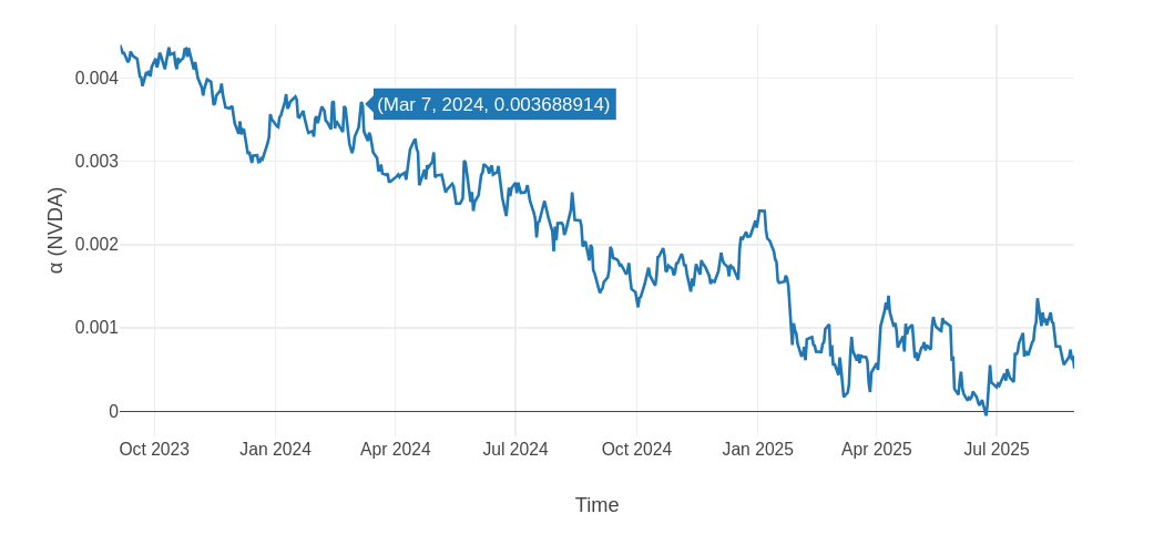
The above charts show the alpha over time for NVDA(Nvidia) and the historical alpha tracking can help inform future trades. A close-up analysis of alpha reveals some interesting observations, for example:
● The declining trend in NVIDIA’s(NVDA) alpha relative to the S&P 500, as observed from October 2023 to July 2025, reflects a significant shift in the stock’s market performance dynamics.
● Initially exhibiting strong positive alpha-indicative of substantial outperformance over the broader market-NVDA’s excess return diminished steadily over time, converging toward zero by mid-2025.
● This erosion of alpha can be attributed to a combination of factors, including the normalization of AI-driven valuation premiums, increased competitive pressures from semiconductor peers, and a broader market environment characterized by robust S&P 500 performance that reduced NVDA’s relative advantage.
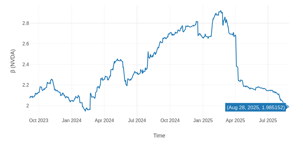
Similarly, the above charts reveals some trends regarding the beta of the NVDA(Nvidia) stock:
● The time series of NVIDIA’s(NVDA) beta relative to the S&P 500 reveals a significant evolution in the stock’s sensitivity to market movements over the period from October 2023 to August 2025.
● Initially, NVDA exhibited a beta around 2.0, indicating that it was approximately twice as volatile as the broader market. Over the course of 2024, beta steadily increased, peaking near 2.9 in early 2025, reflecting heightened market exposure and amplified price swings during periods of strong investor enthusiasm for AI-driven growth.
● This elevated beta suggests that NVDA was behaving as a high-risk, high-reward asset, with returns highly correlated to-and often magnified by-market trends. However, beginning in April 2025, beta experienced a sharp decline, falling to 1.985 by August 2025, signaling a reduction in its volatility relative to the market. This decrease may reflect a combination of factors: valuation corrections, reduced speculative positioning, and a shift toward more stable, earnings-driven investment behavior.
Hence, a portfolio manager when looking at the historical performance of NVDA, will be able to evaluate if the trade is adding value to their portfolio. A stock with a rising alpha and lower beta is a good sign for investment, since it presents a higher return for a lower level of risk. An evaluation of single stocks comprising a portfolio will give a good visual analysis of the stocks risk and return and the overall portfolio. A similar analysis can be conducted at the portfolio level as well to understand the portfolio manager’s performance- alpha creation against the market similar to an AMC tracking a fund’s performance.
5. Discussion
5.1. Toward Reflective Portfolio Management
Rolling alpha and beta are not just statistics-they are mirrors. They allow students to:
● See the consequences of their strategies
● Distinguish luck from skill
● Adjust risk in response to market regimes
5.2. From Classroom to Portfolio Level
This system has direct real-world applicability:
● Can be scaled to real fund management with minimal changes
● Provides a template for risk dashboards in small asset managers
● Integrates with automated compliance or alerting(e.g., “beta increased by 30% this month”)
6. Conclusion
By turning student trades into living data, we move beyond theory to reflective practice. And by building in Clojure, we ensure that the system is not a black box—but an open book. In simple words we can decipher, the best financial models don’t just describe the world—they help people learn from it.
7. Future Work
● Expand to multi-factor rolling models(e.g., FF3: market, size, value)
● Build a web dashboard using ClojureScript(Reagent) for real-time feedback and interactivity
● Implement automated alerts(e.g., “your beta has exceeded 1.5”)
● Add peer benchmarking: compare alpha trajectories across students
● Integrate with portfolio optimization tools for next-step recommendations
● Use the pipeline as a capstone module in investment management courses